Thermal expansion of FeNi Invar and zinc-blende CdTe from the view point of local structure

Introduction

Since the discovery of anomalously large negative thermal expansion (NTE) in ZrW₂O₈ over an extremely wide temperature range in 1996^[1], NTE has revived as a hot topic in structural solid-state chemistry and physics^[2], and novel NTE materials such as Zn(CN)₂ have extensively been reported^[3]. It is essentially important to understand detailed mechanisms of the material function of interest in order to further develop new functional materials. The origin of zero thermal expansion (ZTE) and NTE is known to be categorized into two mechanisms. The first one is a so-called Invar effect, in which the electronic structure of some atoms in the system is temperature dependent. The atomic radius becomes smaller with the temperature rise due to the transformation of the electronic structure, and the Fe₆₅Ni₃₅ Invar alloy^[4] is one of the best examples in this category. The second one is derived from vibrational anomaly. The materials with zinc blende or diamond structure mostly show NTE at low temperature due to the presence of vibrational anomaly^[5]. Well known giant NTE materials such as ZrW₂O₈ and Zn(CN)₂ also belong to this category.

It is well known that thermal expansion is caused by anharmonicity in the interatomic potential, especially the third order^[6]. Although the lattice vibrational dynamics is often approximated within the assemble of harmonic oscillators, anharmonicity must be taken into consideration to account for thermal expansion. Moreover, in order to evaluate thermal expansion quantitatively especially at low temperature, it is essentially important to treat the anharmonic lattice system quantum mechanically. The quantum mechanical anharmonic vibration is usually treated as a perturbation from a harmonic oscillator, and it is well known that the presence of the zero-point vibration drastically makes the quantum effect important at low temperature. In order to describe the finite temperature effect in the lattice dynamics, the quantum statistical perturbation theory should be employed^[7]. Although the quantum statistical perturbation theory can be applied to simple systems such as diatomic molecules, it is too complicated to construct analytical formalism and to perform numerical calculations of the solid NTE and ZTE materials. In real NTE and ZTE systems, computational simulation techniques should be much more suitable rather than analytical formulation methods. A computational simulation technique based on quantum mechanics, which treats quantum mechanical nuclear motion is known as the path integral theory^[7,8]. The path-integral Monte-Carlo simulation method could be ideally the most appropriate to describe anharmonic lattice dynamics at finite temperature. It is however practically still too complicated to evaluate lattice dynamics of complicated solid NTE and ZTE systems. More practical approximation method should be helpful. In 1990s, the path-integral effective classical potential method (PIECP) was developed exactly for the purpose of quantum mechanical anharmonic lattice dynamics and is practically quite useful^[9,10]. In this theory, the path-integral quantum effect is included as a correction in the classical Monte-Carlo simulations, and we do not have to perform complicated quantum mechanical path integral calculations, being suitable to mostly describe thermal expansion of normal solids at low temperature.

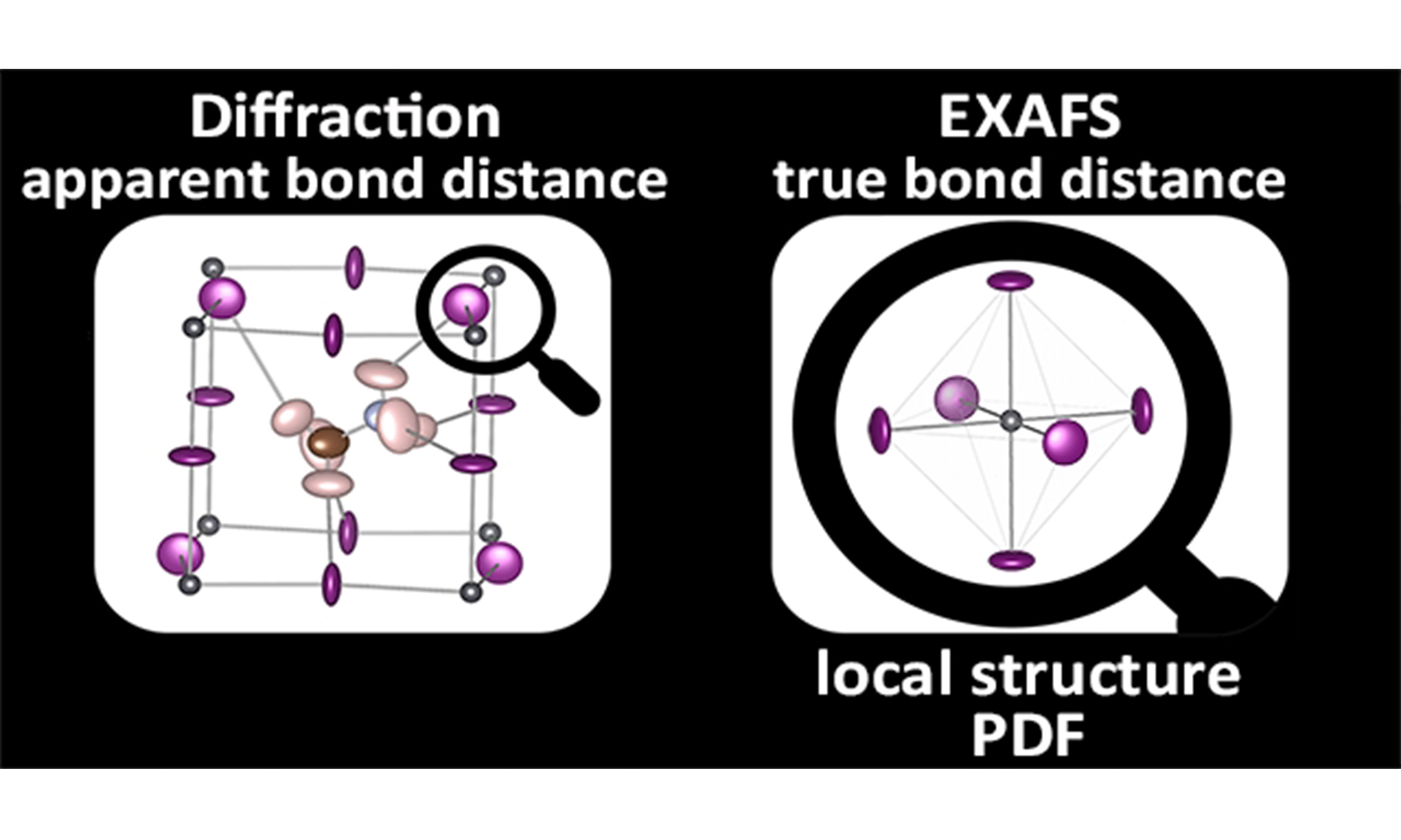
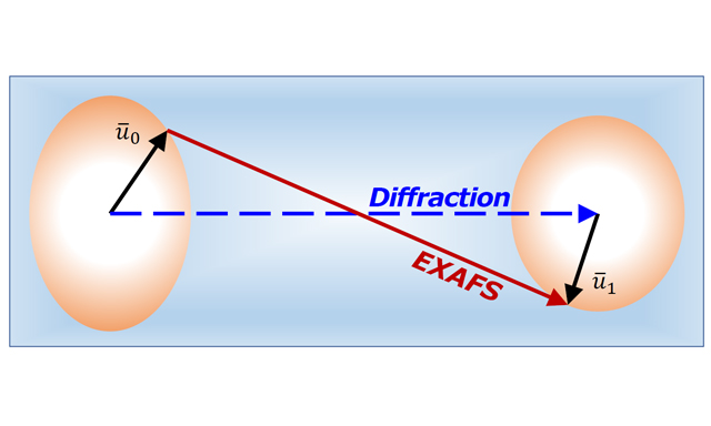
The other concept other than the quantum effect in the present article is a local point of view in thermal expansion. Although thermal expansion itself is a macroscopic character, there can be seen several essential differences in thermal expansion between microscopic and macroscopic geometrical structures. In disordered alloy systems such as the Invar alloy, although the x-ray diffraction often exhibits simple crystal structure like fcc, different atomic pairs give different interatomic distances. In case of the Fe₆₅Ni₃₅ Invar alloy, the crystal structure looks simple fcc, while the interatomic distances are not equivalent among Fe-Fe, Fe-Ni, and Ni-Ni pairs. In zinc blende materials as well, the first nearest neighbor (NN) interatomic distance does not correspond to the equilibrium distance calculated from the lattice constant, due to the presence of vibrational motion perpendicular to the bond direction at the equilibrium geometry. In order to reveal the local structure, especially to clarify the difference between the local structure and the equilibrium crystal structure, extended x-ray-absorption fine structure (EXAFS) spectroscopy is quite useful^[11,12]. The EXAFS method provides detailed information on anharmonicity or asymmetric radial distribution quantitatively.

Let us here briefly review the EXAFS spectroscopy for anharmonic lattice dynamics from the historical point of view. In the conventional EXAFS formula, a narrow Gaussian function is assumed for the radial distribution function around x-ray absorbing atom. Although this approximation is often appropriate and is assumed even in the present standard EXAFS analysis, erroneous results such as too short interatomic distances would be obtained in the analysis of a large anharmonic system. This caution was firstly pointed out by Eisenberger and Brown^[13], and subsequently a general formulation using cumulant expansion was proposed by Bunker^[14]. In the cumulant expansion, the radial distribution function is parametrized as cumulant moments up to the third or fourth order (up to the second-order expansion corresponds to the conventional Gaussian approximation), which will be given in detail in the next section. It is now recognized that appropriate consideration of the EXAFS cumulants (usually up to the third- or fourth-order cumulants) will advantageously provide additional important information on anharmonicity of the lattice vibration, rather than disadvantage of the EXAFS technique.

Theoretical formulation of the EXAFS cumulants has also been developed. The classic statistical dynamics theory easily provides the EXAFS cumulants assuming the Boltzmann distribution function, although the overall potential in the solid is rather complicated even in the case of summation of two-body interatomic potentials^[15]. Frenkel and Rehr^[16] showed the third-order EXAFS cumulant expression for a diatomic molecule using the quantum statistical first-order perturbation theory. More recently, Yokoyama^[17,18] similarly derived the fourth-order EXAFS cumulant for a diatomic molecule using the quantum statistical second-order perturbation theory. Although the EXAFS cumulants obtained in this theory can be applied to rather simple polyatomic systems as triatomic^[19], octahedral^[20], and tetrahedral^[21] molecules and a one-dimensional infinite chain^[22], it is too complicated to adopt anharmonic vibration of crystalline solids, as mentioned above. Fujikawa et al.^[23] firstly applied the PIECP method for the theoretical description of the EXAFS cumulants, where the one-dimensional chain system was again examined. Subsequently, Yokoyama^[24,25] utilized the PIECP method to describe practical three-dimensional crystalline system. This extension allows one to apply the PIECP method to the ZTE and NTE materials rather straightforwardly.

In the present article, we will focus our attention on the quantum effect and the local structural point of view for thermal expansion, especially for the understanding of ZTE and NTE. We will recognize that these effects are quite important for thermal expansion phenomena of ZTE and NTE materials. In the subsequent section, after the definition of the EXAFS cumulants, the quantum statistical perturbation theory is intuitively recalled to understand thermal expansion in detail. Differences in thermal expansion between the quantum mechanical and classical theories is emphasized. The analytical formulas for the EXAFS cumulants will be a great help to recognize the relationship between the local and macroscopic average thermal expansion. The other anharmonicity of temperature dependent elasticity (softening with a temperature rise) is also discussed briefly. As an example, the experimental Br K-edge EXAFS result of diatomic Br₂ is presented and comparatively discussed in the quantum statistical second-order perturbation theory. In a subsequent section, the path-integral effective classical theory is described. It is here important for readers to understand advantages and disadvantages in this theoretical calculation, because the method contains many approximations to realize numerical simulations with low computational cost.

In the next section, the local thermal expansion of the FeNi Invar alloy is discussed by using the experimental Fe and Ni K-edge EXAFS spectra, together with the PIECP and classical Monte Carlo (MC) computer simulations. The contributions of the quantum effect and the different atomic pairs to thermal expansion are elucidated. Subsequently, the local thermal expansion of CdTe is discussed by using the experimental Cd and Te K-edge EXAFS spectra, together with the PIECP and classical MC computer simulations. The origin of negative thermal expansion in these tetrahedral crystals is known as a result of classical vibrational anomaly that can be described within the Newton dynamics theory. In spite of that, the quantum statistical simulation is found to be essentially indispensable to reproduce the negative thermal expansion of CdTe appropriately. Finally, in the last section, the present review will be conclusively summarized and some perspectives on future directions will be discussed including the role of microstructures of the materials.

Quantum statistical perturbation theory

Diatomic bromine molecule

Figure 1 shows the Morse potential of diatomic Br₂, where D_e = 2.113 (eV), α = 0.1661 (nm), and r_e = 0.2284 (nm) in eq. (4)^[26]. The light-blue lines correspond to the eigenstates exactly obtained by solving the Schrödinger equation. The black dot denotes the average interatomic distance at each eigenstate. It is easily understandable that the interatomic distance becomes longer as the eigenenergy increases, implying the occurrence of the thermal expansion in diatomic Br₂. The force constants in eq. (3) are given as κ₀ = 2.459 × 10² (N/m), κ₃=1.756 × 10¹² (N/m²) and κ₄=1.058 × 10²² (N/m³).

Figure 1. Morse potential of diatomic Br₂. The thin light-blue lines correspond to the eigenstates, and the black dots to the average interatomic distance for each eigenstate.

Figure 2 gives the experimentally obtained EXAFS cumulants C₂, C₃, and C₄ of diatomic Br₂ by measuring temperature dependent Br K-edge EXAFS spectra of gaseous Br₂, together with the calculated theoretically using eqs. (9-13)^[17,18]. Agreements between the experiment and the calculation are fairly good. It is noted that C_2,qu shows nonzero value at T = 0 due to harmonic zero-point vibration. C_3,qu also exhibits nonzero value at T = 0, although the difference between the quantum and classical results is much smaller than in C₂. Experimental C₄ is found to be positive, implying that the second-order perturbation term originating from the third-order force constant $$ \kappa_{3}^{2} $$ dominantly contributes to C₄.

Figure 2. EXAFS cumulants (A) C₂, (B) C₃, and (C) C₄ of diatomic Br₂. The blue points with error bars are the experimental cumulants determined by the Br K-edge EXAFS analysis, while the red and green lines are the theoretical ones calculated by the quantum statistical perturbation theory [eqs. (9-11)] and by the classical limit [eqs. (12,13)].

Figure 3 shows the theoretically calculated thermal expansion and temperature dependent effective force constants. Thermal expansion exhibits a similar behaviour to C_2,qu, as expected in eqs. (9) and (12). At low temperature, the deviation between the two lines is enlarged, and even at T = 0, the quantum result exhibits elongation with respect to r₀ due to the finite zero-point vibrational amplitude, while the classical result yields a linear function exactly proportional to T. The decrease in the effective force constant with a temperature rise implies the vibrational softening due to the third- and fourth-order anharmonic force constants. The classical result shows a linear decrease, while the quantum result exhibits a concave feature as in thermal expansion. From positive C₄ in Figure 2, the second-order perturbation due to the third-order force constant is concluded to be a dominant contribution to the temperature dependence of the effective force constant (vibrational softening).

Figure 3. (A) Thermal expansion R - r₀ and (B) effective force constant k_eff of diatomic Br₂, calculated by the quantum statistical perturbation theory and by the classical limit.

Path integral effective classical potential theory

Invar alloy

Anomalously small thermal expansion over a wide temperature range in an iron-nickel alloy with a nickel concentration of around 35% was discovered by Guillaume^[4] in 1897. Figure 4 shows temperature dependence of the interatomic distance and Young moduli of typical metals. The Fe₆₅Ni₃₅ Invar alloy actually exhibits almost ZTE, while stainless steel (SUS304, Fe₇₂Ni₉Cr₁₈Mn₁) gives much larger normal thermal expansion. Interestingly, in Figure 4B, the Invar alloy shows an increase in the Young modulus with the temperature rise, which is essentially different from other normal metals as SUS304, Ni, and Cu. In Figure 4, the behaviours of Ni Span C (Fe₅₀Ni₄₂Cr₆Ti₄) are also given, which is sometimes called the Elinvar alloy exhibiting almost no temperature dependence of the elastic constant, accompanied by smaller thermal expansion. The Invar and Elinvar alloys have been utilized in various kinds of industrial products.

Figure 4. Temperature dependence of (A) the first NN interatomic distances of the Invar (purple line, Fe₆₅Ni₃₅), stainless steel SUS304 (blue points, Fe₇₂Ni₉Cr₁₈Mn₁), and Ni Span C (red line, Fe₅₀Ni₄₂Cr₆Ti₄) alloys, and Cr, Fe, Ni, and Cu elemental metals, and (B) the Young moduli of the Invar, SUS304, and Ni Span C alloys, and Ni, and Cu elemental metals^[34].

The ZTE behaviour of Fe₆₅Ni₃₅ is well known as a result of the so-called Invar effect. Other physical properties such as elastic constants and magnetization show also anomalous behaviours^[35-38]. A basic concept of the Invar effect is that there exist at least two types of electronic states in Fe, typically high-spin (HS) and low-spin (LS) states. In this two-state model, the equilibrium potential energy is lower in the HS state than in the LS one, while the equilibrium atomic radius is larger in the former. This results in the compensation of thermal expansion due to increasing density of the LS state at higher temperature. A recent ab initio electronic structure calculation at 0 K, however, suggests much more complicated electronic configurations in a smaller volume region^[39]. Computational simulations at finite temperatures have also been carried out for the understanding of magnetization and thermal expansion^[40-44].

In this section, let us see the experimental and computational results of the local thermal expansion and the anharmonic behaviour^[45]. Temperature dependent Fe and Ni K-edge EXAFS spectra of the Fe₆₅Ni₃₅ Invar alloy were recorded using synchrotron radiation (Photon Factory, Tsukuba, Japan) and the MC simulation results based on the PIECP and classical theories within the simple two-state (HS + LS) model. Since we discuss thermal expansion, the MC simulations were performed under a constant pressure condition (NPT condition). 500 atoms (5³ fcc cubic unit cells) were employed and the distributions of Fe and Ni were chosen randomly. Eleven types of the superlattices were simulated and the results were averaged to provide consequent physical quantities.

Figure 5 shows the first NN interatomic distances around Fe and Ni obtained by the experimental EXAFS analysis^[45] and the lattice constant given by the X-ray diffraction^[46], together with those simulated by the PIECP and classical MC methods. Figure 5A gives the potential energies of Invar Fe₆₅Ni₃₅ and fcc Fe at T = 0 as a function of the first NN distance. In the present atomic potentials, the fcc Fe system shows that the LS state is slightly more stable by 8.0 meV than the HS state with R_HS = 0.2530 (nm) and R_LS = 0.2492 (nm), while the Invar case exhibits a more stable HS state by 25.0 meV with R_HS = 0.2530 (nm) and R_LS = 0.2490 (nm). In Figure 5B-D, the agreement between the PIECP and experiments is fairly good: almost no thermal expansion around Fe and small but meaningful thermal expansion around Ni. On the contrary, the classical method is found to give fatal discrepancy at low temperature below ~100 K; the interatomic and lattice distances significantly increase with the temperature rise. These findings imply the essential importance of the quantum effect, which is recognized as a result of zero-point vibration.

Figure 5. (A) Average potential energies of the Invar (top lines), fcc Fe (bottom lines), and fcc Ni (bottom, green dotted line) as a function of the first NN distance at T = 0. For Fe, two types of the potentials for the HS (red solid line) and LS (blue dashed line) states are depicted. (B, C) Simulated first NN interatomic distance around Fe (B) and Ni (C) given by the PIECP (blue circles and solid line, quantum) and the classical MC (green diamond and dashed line, classic) methods, together with the experimental EXAFS data (red open circle with an error bar). (D) Equilibrium first NN distance (a₀/√2) given by the PIECP and classical MC simulations, together with the experimental literature data^[44].

To get further insights into local thermal expansion, the first NN interatomic distance of each component (Fe-Fe, Ni-Ni and Ni-Fe) pair is shown in Figure 6. In this plot, the PIECP MC results, by using only the HS Fe state, are also depicted to recognize hypothetical normal thermal expansion in this system. As expected, the Fe-Fe pair shows the largest discrepancy between the two-state (HS + LS) and the HS-only models. This is caused by the increasing population of the Fe LS state with the temperature rise, yielding compensation of thermal expansion with the one originating from anharmonic vibration. The most important finding in Figure 6 is that even Ni-Ni and Ni-Fe pairs exhibit significant suppression of thermal expansion. This is consistent with the above experimental finding that thermal expansion around Ni is noticeably suppressed compared to that of fcc Ni. Although Ni does not change its electronic configuration depending on temperature and may tend to expand because of anharmonic vibration, the Ni-Ni or Ni-Fe expansion is significantly suppressed due to the anomalously small expansion of the lattice. Interestingly, the suppression of thermal expansion seems more significant in the Ni-Fe pair than in the Ni-Ni one. This can be explained by the fact that the Fe atom surrounded by many Ni atoms tends to maintain the HS state. In the present EAM potentials, the energy difference between the HS and LS states is determined by the sum of the d electron density of surrounding atoms at the Fe site. Although the number of the d electrons of Ni is larger than that of Fe, the d electron density at the first NN distance is smaller in Ni than in Fe because of larger nuclear charge in Ni and thus less delocalized electronic cloud in Ni. This leads to stabilization of the ferromagnetic exchange interaction of Fe and thus more probability of the HS state surrounded by more Ni atoms. Furthermore, the Ni-Ni interaction is noticeably softer than the Ni-Fe one and is more likely to match the lattice parameter. These effects consequently yield smaller thermal expansion in the Ni-Ni pair than the Ni-Fe one.

Figure 6. Simulated first NN interatomic distances of Fe-Fe (blue square and solid line), Ni-Ni (red square and solid line), and Ni-Fe (green square and solid line) pairs, together with the average ones around Fe (pink circle and solid line) and Ni (orange circle and solid line). The experimental data for the average one around Fe and Ni are also shown. The dashed lines are the PIECP results by using only the HS state in Fe^[44].

Let us also discuss the third-order anharmonicity in the Invar alloy. Figure 7 shows C₃ for the average first NN shells around Fe and Ni, respectively. The agreement between the experiments and the PIECP simulations is not perfect, but C₃ increases gradually with the increase in temperature for both the Fe and Ni data. Clear anharmonicity in the Invar alloy is confirmed by comparing the PIECP simulations between the two-state (HS + LS) and HS-only models. Both the simulated data exhibit essentially the same C₃ values, implying no suppression of C₃ due to the contribution of the LS state, as observed in the thermal expansion. Since the asymmetric radial distribution for the first NN shell almost exclusively originates from the anharmonic interatomic potential, the present result implies that the third-order anharmonicity clearly exists even in the case of no thermal expansion. Note that in the present PIECP simulations within the low coupling approximation, the quantum effect in C₃ is not properly taken into consideration because of the neglect of the phonon-phonon coupling. The important qualitative finding of the presence of C₃ without thermal expansion is, however, clearly exemplified.

Figure 7. The third-order EXAFS cumulant C₃ given by the experimental EXAFS (red open circle with an error bar) and by the PIECP simulations using the two-state (blue circle and dashed line) and the HS-only (green solid line) models for the average first NN distribution around (A) Fe and (B) Ni^[44].

At the end of this section, the interatomic potentials around Fe are summarized in Figure 8 to compare between the three different Fe-based alloys of the Invar (Fe₆₅Ni₃₅), SUS316L (Fe₆₇Cr₁₈Ni₁₂Mo₂Mn₁)^[47], and Elinvar (Fe₅₀Ni₄₂Cr₆Ti₄)^[34] alloys. The stainless steel SUS316L alloy exhibits normal thermal expansion that is quantitatively almost the same as that of SUS304 in Figure 4A. The Elinvar (Ni Span C) alloy shows intermediate thermal expansion as shown in Figure 4A due to the partial Invar effect. In the Invar alloy, the HS state of Fe is located below the LS state, ΔE ≡ E_LS-E_HS = 0.034 (eV), and the LS state gives a shorter interatomic distance of R_LS = 0.2512 (nm) and a stiffer bulk modulus of B_LS = 182 (GPa) than those of the LS state with R_HS = 0.2553 (nm) and B_HS = 147 (GPa) (Note here that the potential parameters are slightly different from those in Figure 4). Since the energy difference between the HS and LS states is not so large compared to the thermal energy, the population of the LS state increases gradually with the temperature rise, yielding the compression of the interatomic distance that compensates for the thermal expansion due to anharmonicity and the enlargement of the bulk modulus. The enlargement of the elastic constant is an interesting peculiar character compared to normal metals that show the softening of the elastic constant.

Figure 8. Potential diagrams around Fe atoms in (A) Invar (Fe₆₅Ni₃₅), (B) SUS316 (Fe₆₇Cr₁₈Ni₁₂Mo₂Mn₁), and (C) Elinvar (Fe₅₀Ni₄₂Cr₆Ti₄) alloys. FM and NM denote the ferromagnetically coupled high-spin and nonmagnetic low-spin Fe, respectively^[47].

On the contrary, SUS316L shows that the HS state of Fe is located DE = -0.095 (eV) above the LS state, and the LS state gives a shorter interatomic distance of R_LS = 0.2544 (nm) and a stiffer bulk modulus of B_LS = 177 (GPa) than those of the HS state with R_HS = 0.2549 (nm) and B_HS = 143 (GPa). A much larger energy difference between the LS and HS states does not induce noticeable thermal excitation, leading to normal thermal expansion and elasticity softening of SUS316L at high temperature. In case of the Elinvar alloy, the situation is more complicated. There exist two types of Fe atoms, the one of which gives more unstable LS state [LS1: ΔE = 0.053 (eV), R_LS = 0.2520 (nm), B_LS = 175 (GPa)] than the HS state [HS1: R_HS = 0.2559 (nm) B_HS = 143 (GPa)] as in the case of the Invar alloy, and the other of which exhibits more stable LS state [LS2: ΔE = -0.134 (eV), R_LS = 0.2516 (nm), B_LS = 173 (GPa)] than the HS state [HS2: R_HS = 0.2533 (nm) B_HS = 131 (GPa)] as in the case of the SUS316 alloy. These findings imply that some Fe shows the Invar effect, while the other does the anti-Invar effect, resulting in an incomplete Invar effect in the Elinvar alloy. Such a different behavior in the Fe atoms is attributed to different coordination around Fe. Fe is surrounded by 35% Ni in the Invar alloy, and by 18% Cr and 12% Ni in the SUS316L. In the EAM scheme, surrounding Cr is likely to stabilize the LS state of Fe, while Ni is to stabilize the HS state of Fe, because the Cr 3d electrons are much more delocalized and interact more strongly with Fe 3d than the Ni one due to the difference in the nuclear charge. In the Elinvar alloy, Fe is surrounded by 42% Ni, 6% Cr and 4% Ti, yielding coexistence of more stable HS and LS states in Fe, depending on the coordination of Ni or Cr and Ti.

Other related works concerning the local thermal expansion and the elastic constant using experimental EXAFS analysis combined by the PIECP computational simulation can be found in literatures: solid Kr^[48], martensitic Mn₈₈Ni₁₂ alloy^[49] and (Zr,Nb)Fe₂^[50]. At the end of this section, a sophisticated hot article published very recently is cited^[51], which gives the experimental EXAFS results of the FeNi Invar alloy at extremely high pressure including the magnetic phase transition.

Zinc blende

Most zinc blende and diamond structure materials show NTE at low temperature, except diamond. The mechanism of the NTE in these tetrahedral materials is rather simple and seems well established already. Let us consider the transverse acoustic phonon mode around the X point in the first Brillouin zone in diamond or zinc-blend structure, as shown in Figure 9. Assuming that the phonon propagating direction is along the [001] axis and the vibrational direction of atoms is [110], the mode yields a vibrational motion between atoms 1 and 2 perpendicular to the bond direction (see Figure 9B). In this situation, the equilibrium distance between atoms 1 and 2, R₀ in the left of Figure 9C, is forced to be the shortest bond length. This lattice configuration is unstable because the force between atoms 1 and 2 is always attractive as long as the equilibrium distance corresponds to the natural length of the spring, consequently leading to lattice contraction to provide the most stable lattice constant depending on the vibrational amplitude of the phonon mode as in the right panel of Figure 9C. This NTE model has extensively been discussed since the first discovery of NTE in Si^[5]. More recently, the first-principles DFT calculations concerning the NTE of Si were performed^[52]. Although in the electronic structure calculations the Si atoms move classically, they applied the quantum mechanical quasi-harmonic approximation to the lattice dynamics and elucidated a negative Grüneisen constant and a resultant NTE at low temperature. It should be noted here that the mechanism of the NTE is purely classic, although the term of phonon is used for convenience, because the lattice instability due to the vibration perpendicular to the chemical bond, as discussed above, can be described completely within the classical Newton equation of motion in the lattice dynamics theory.

Figure 9. Schematic mechanism of the NTE in zinc-blend structure. (A) A cubic unit cell of zinc blende structure, (B) schematic view of the transverse acoustic vibrational mode around the X point in the Brillouin zone, and (C) look of atoms 1 and 2 along the axis. In (B), the vibrational motions of atoms 1 and 2 are in antiphase. In (C), R₀ and R (R₀’ and R’) in the left (right) are initial (relaxed) equilibrium and instantaneous interatomic distances, respectively. Due to the vibrational instability, the lattice is consequently contracted.

More recently, Dalba and Fornasini group performed systematic investigations concerning NTE in tetrahedral and other systems using EXAFS spectroscopy quite in detail^[53-57]. They observed excellently significant discrepancies between the interatomic distance given by EXAFS and the equilibrium distance (lattice constant) given by XRD, where the interatomic distances show quite normal thermal expansion as in ordinary materials with positive thermal expansion. This discrepancy is however straightforwardly understandable from the above discussion, because in the presence of sufficiently large vibrational amplitude perpendicular to the chemical bond the interatomic distance is always larger than the equilibrium distance, as seen in Figure 9C. They successfully derived the vibrational amplitude perpendicular to the bond from the interatomic distances, which was found to be several times larger than the one parallel to the bond. The origin of the NTE in tetrahedral systems is well understood more quantitatively through the experiments.

In this study, to realize the NTE of zinc-blend structure computationally, classical and quantum mechanical simulations have been performed for CdTe. There have been no reports concerning classical or quantum mechanical lattice dynamics simulations for the NTE in diamond or zinc-blend structure to the best of the author’s knowledge. As discussed above, the mechanism of the NTE can thoroughly be described within the classical dynamics theory, and the NTE in CdTe should be reproduced by the classical MC simulations. Classical and PIECP MC simulations have been performed under the NPT condition with the total number of atoms N = 512 (4³ cubic unit cells). The bond-order potential (BOP)^[58,59] of CdTe reported recently in the literature^[60] is sufficiently reliable for the present investigation and was used without any modification.

Figure 10 shows temperature dependence of the calculated interatomic distances in CdTe, together with the experimental results of EXAFS^[55,56] and XRD^[46]. The distances are scaled to match the first NN Cd-Te one; for instance, the lattice constant is multiplied by √3/4. The XRD result shows the NTE of the lattice constant between 20 and 80 K, while the EXAFS result exhibits rather normal thermal expansion with larger temperature dependence even at higher temperature. The calculated result using the classical dynamics provides almost linearly increasing thermal expansion. Although the classical dynamics may expect the NTE in CdTe as mentioned above, it is clarified that the NTE cannot be realized within the classical theory. On the contrary, the PIECP result exhibits the NTE at low temperature, implying semiquantitative agreement with the XRD experiment. Moreover, the calculated first-NN interatomic distance shows rather normal thermal expansion, which is also in semiquantitative agreement with the EXAFS experiment. As the shell is going to higher neighbors, the temperature dependence is gradually suppressed and approaches the lattice behavior. It is strikingly concluded that vibrational quantum fluctuations are essentially required to realize the NTE in CdTe, although the NTE mechanism is purely classic. It is here noted that similar simulations have been performed for diamond and CdSe, which are found to exhibit positive and negative thermal expansions, respectively, also in qualitative agreement with the experimental findings.

Figure 10. Calculated temperature dependence of the distances in CdTe, together with the experimental XRD (light blue solid circle)^[46] and EXAFS (orange open circle)^[55,56] results. The lattice constant (black), the first (red), second (green), third (blue), and fourth (magenta) NN distances are depicted, obtained by the PIECP (solid) and classical (dashed) MC simulations. All the distances are scaled to match the first NN distances.

Figure 11 shows temperature dependence of the mean square relative displacements for the first to third NN shells in CdTe obtained by the lattice dynamics calculations within the harmonic approximation, together with the EXAFS results. Both the components parallel and perpendicular to the corresponding atom pairs are depicted (parallel component corresponds to C₂). It is found that in the first NN Cd-Te shell the perpendicular MSRD is much larger than the parallel one due to the presence of strong chemical bond between Cd and Te, semiquantitatively consistent with the experimental findings. The large perpendicular MSRD may result in normal local thermal expansion for the first NN Cd-Te distance in spite of the NTE for the lattice constant. The second NN shell exhibits smaller difference between the parallel and perpendicular components due to the absence of the direct chemical bonds in the second NN shell. Note here that although there exist two kinds of the second NN shells of Cd-Cd and Te-Te, the difference is found to be negligibly small and only the Cd-Cd calculated results are depicted in Figure 11. The third NN shell gives almost identical MSRD between the parallel and perpendicular components, implying no anisotropic correlated motions in higher NN shells because of almost no interactions in the third NN shell.

Figure 11. (A) Temperature dependence of the first-NN MSRD parallel (red) and perpendicular (blue) to the Cd-Te bond, obtained by the lattice dynamics calculations within the quantum mechanical (solid lines) and classical (dashed lines) harmonic approximations, together with the experimental EXAFS (symbols) results^[55,56]. (B) Temperature dependence of the second (green) and third (blue) NN MSRD parallel (solid lines) and perpendicular (dashed lines) to the atomic pair direction, together with the experimental EXAFS (symbols) results for the parallel components. The perpendicular component is divided by 2 to compare with the parallel one directly.

The most striking consequence in this work is that vibrational quantum fluctuation is essentially important to realize the NTE, although the mechanism of the NTE is well established and is regarded as a purely classical origin. In the classical model, normal vibrational modes such as stretching modes with higher frequencies that contribute to positive thermal expansion dominate the lattice potential, because the vibrational excitations take place irrespective of the vibrational frequencies in the classical theory. The vibrational amplitude perpendicular to the chemical bond, which is a key role of the NTE and was experimentally given by the previous sophisticated EXAFS works, is successfully reproduced in the present computational study. Other thermal properties such as bulk moduli and higher-order anharmonicity (EXAFS cumulants) show quite normal behaviors, which are also reasonably and reliably understood in the present simulations.

Conclusions

In this article, fundamental quantum mechanical theories of thermal expansion were at first described in the quantum statistical perturbation and path-integral frameworks. The EXAFS cumulants that characterize thermal vibration and thermal expansion are formulated using the Br K-edge EXAFS of diatomic Br₂ as a practical experimental example. The importance of the quantum effect is exemplified for the description of the low-temperature thermal properties such as thermal expansion. Subsequently, zero thermal expansion of FeNi Invar and negative thermal expansion of zinc-blende CdTe were discussed from the view point of local structure. These two examples exhibit anomalous thermal expansion due to different origins of the so-called Invar effect (temperature variation of electronic structure) and vibrational anomaly. The local thermal expansion is discussed based on experimental EXAFS spectroscopic data and the path-integral effective classical potential (PIECP) Monte Carlo computational simulations.

In the FeNi Invar alloy, in which zero thermal expansion is seen over a wide temperature range including very low temperature, the vibrational quantum effect is found to be essentially important; quantum mechanical thermal expansion tends to be zero at the absolute temperature, while classic mechanically thermal expansion is constant, irrespective of temperature. It is also noted that the interatomic distances and thermal expansion of different atomic pairs (Fe-Fe, Fe-Ni, and Ni-Ni in the FeNi Invar alloy) are slightly but meaningfully different from each other, although the alloy exhibit a simple fcc crystal. Moreover, the third-order anharmonicity is found to be present as in normal metals, although usually the third-order anharmonic force constant is believed to be proportional to the thermal expansion coefficient. In the zinc blende and diamond structures, the origin of negative thermal expansion in these tetrahedral crystals is known as a result of classical vibrational anomaly within the Newton dynamics theory. The quantum statistical simulation is however found to be essential to reproduce the negative thermal expansion of CdTe.

Finally, let us briefly discuss some perspectives on future directions of EXAFS spectroscopy for the investigation of thermal properties of the materials such as ZTE and NTE. Since the synchrotron radiation techniques have substantially been developed in recent years and are still being exploited, especially for the three-dimensional spectromicroscopic computer-tomographic imaging method. It is essentially important to investigate structures within single domains and also their grain boundaries not only in the magnetic ZTE and NTE materials but also in other functional materials including multi-phase materials that exhibit interesting thermal and other physical/chemical properties. The spatial resolution of the computer-tomographic EXAFS imaging may reach less than 10 nm, leading to visualization of three-dimensional crystal and local atomic-scale structure of functional materials in near future.

REFERENCES

1. Mary TA, Evans JSO, Vogt T, Sleight AW. Negative thermal expansion from 0.3 to 1050 Kelvin in ZrW2O8. Science 1996;272:90-2.
2. Chen J, Hu L, Deng J, Xing X. Negative thermal expansion in functional materials: controllable thermal expansion by chemical modifications. Chem Soc Rev 2015;44:3522-67.
3. Chapman KW, Chupas PJ, Kepert CJ. Direct observation of a transverse vibrational mechanism for negative thermal expansion in Zn(CN)2: an atomic pair distribution function analysis. J Am Chem Soc 2005;127:15630-6.
5. Blackman M. On the thermal expansion of solids. Proc Phys Soc 1957;70:827-32.
6. Kittel C. Introduction to solid state physics. 8th ed. Wiley; 2004.
7. Feynman RP. Statistical Mechanics: a set of lectures. Reading, MA: Benjamin; 1972.
8. Kleinert H. Path Integrals in Quantum Mechanics, Statistics and Polymer Physics and Financial Markets. Singapore: World Scientific; 1995.
9. Cuccoli A, Macchi A, Neumann M, Tognetti V V, Vaia R. Quantum thermodynamics of solids by means of an effective potential. Phys Rev B Condens Matter 1992;45:2088-96.
10. Cuccoli A, Giachetti R, Tognetti V, Vaia R, Verrucchi P. The effective potential and effective Hamiltonian in quantum statistical mechanics. J Phys Condens Matter 1995;7:7891-938.
11. Sayers DE, Stern EA, Lytle FW. New technique for investigating noncrystalline structures: Fourier analysis of the extended X-Ray - absorption fine structure. Phys Rev Lett 1971;27:1204-7.
12. Bunker G. Introduction to XAFS: A Practical Guide to X-ray Absorption Fine Structure Spectroscopy. Cambridge: Cambridge University Press; 2010.
13. Eisenberger P, Brown GS. The study of disordered systems by EXAFS: Limitations. Solid State Commun 1979;29:481-4.
14. Bunker G. Application of the ratio method of EXAFS analysis to disordered systems. Nucl Instrum Method Phys Res 1983;207:437-44.
15. Yokoyama T, Satsukawa T, Ohta T. Anharmonic interatomic potentials of metals and metal bromides determined by EXAFS. Jpn J Appl Phys 1989;28:1905-8.
16. Frenkel AI, Rehr JJ. Thermal expansion and x-ray-absorption fine-structure cumulants. Phys Rev B Condens Matter 1993;48:585-8.
17. Yokoyama T. Path-integral effective-potential theory for EXAFS cumulants compared with the second-order perturbation. J Synchrotron Radiat 1999;6:323-5.
18. Yokoyama T. Path-integral approach to anharmonic vibration of solids and solid interfaces. J Synchrotron Radiat 2001;8:87-91.
19. Yokoyama T, Kobayashi K, Ohta T, Ugawa A. Anharmonic interatomic potentials of diatomic and linear triatomic molecules studied by extended x-ray-absorption fine structure. Phys Rev B Condens Matter 1996;53:6111-22.
20. Yokoyama T, Yonamoto Y, Ohta T, Ugawa A. Anharmonic interatomic potentials of octahedral Pt-halogen complexes studied by extended x-ray-absorption fine structure. Phys Rev B Condens Matter 1996;54:6921-8.
21. Yokoyama T, Yonamoto Y, Ohta T. Anharmonicity of the bending and stretching vibrations observed in extended X-ray absorption fine structure of tetrahedral molecules. J Phys Soc Jpn 1996;65:3901-8.
22. Miyanaga T, Fujikawa T. Quantum statistical approach to Debye-Waller factor in EXAFS, EELS and ARXPS. II. Application to one-dimensional models. J Phys Soc Jpn 1994;63:1036-52.
23. Fujikawa T, Miyanaga T, Suzuki T. Quantum statistical approach to Debye-Waller factors in EXAFS, EELS and ARXPS. V. Real space approach to one-dimensional systems. J Phys Soc Jpn 1997;66:2897-906.
24. Yokoyama T. Path-integral effective-potential method applied to extended x-ray-absorption fine-structure cumulants. Phys Rev B 1998;57:3423-32.
25. Yokoyama T. Fluctuating paths and fields. In: Janke W, Pelster A, Bachmann M, Schmidt HJ, editors. Path-integral and perturbation methods for Debye-Waller factors observed by extended x-ray-absorption fine structure spectroscopy. Singapore: World Scientific; 2001. pp. 337-46.
27. Beni G, Platzman PM. Temperature and polarization dependence of extended x-ray absorption fine-structure spectra. Phys Rev B 1976;14:1514-8.
28. Daw MS, Baskes MI. Embedded-atom method: Derivation and application to impurities, surfaces, and other defects in metals. Phys Rev B 1984;29:6443-53.
29. Foiles SM. Application of the embedded-atom method to liquid transition metals. Phys Rev B Condens Matter 1985;32:3409-15.
30. Foiles SM. Calculation of the surface segregation of Ni-Cu alloys with the use of the embedded-atom method. Phys Rev B Condens Matter 1985;32:7685-93.
31. Foiles SM, Baskes MI, Daw MS. Embedded-atom-method functions for the fcc metals Cu, Ag, Au, Ni, Pd, Pt, and their alloys. Phys Rev B Condens Matter 1986;33:7983-91.
32. Jacobsen KW, Norskov JK, Puska MJ. Interatomic interactions in the effective-medium theory. Phys Rev B Condens Matter 1987;35:7423-42.
33. Ercolessi F, Parrinello M, Tosatti E. Simulation of gold in the glue model. Philosophical Magazine A 1988;58:213-26.
34. Yokoyama T, Koide A, Uemura Y. Local thermal expansions and lattice strains in Elinvar and stainless steel alloys. Phys Rev Materials 2018;2.
38. Matsui M, Chikazumi S. Analysis of anomalous thermal expansion coefficient of Fe-Ni Invar alloys. J Phys Soc Jpn 1978;45:458-65.
39. van Schilfgaarde M, Abrikosov IA, Johansson B. Origin of the Invar effect in iron-nickel alloys. Nature 1999;400:46-9.
40. Rancourt DG, Dang M. Relation between anomalous magnetovolume behavior and magnetic frustration in Invar alloys. Phys Rev B Condens Matter 1996;54:12225-31.
41. Wesselinowa JM, Ivanov IP, Entel P. Localized-magnetic-moment theory of Fe-Ni Invar. Phys Rev B 1997;55:14311-7.
42. Meyer R, Entel P. Martensite-austenite transition and phonon dispersion curves of Fe1-xNix studied by molecular-dynamics simulations. Phys Rev B 1998;57:5140-7.
43. Lagarec K, Rancourt DG. Fe3Ni-type chemical order in Fe65Ni35 films grown by evaporation: implications regarding the Invar problem. Phys Rev B 2000;62:978-85.
44. Gruner M, Meyer R, Entel P. Monte Carlo simulations of high-moment - low-moment transitions in Invar alloys. Eur Phys J B 1998;2:107-19.
45. Yokoyama T, Eguchi K. Anharmonicity and quantum effects in thermal expansion of an Invar alloy. Phys Rev Lett 2011;107:065901.
46. Touloukian YS, Kirby RK, Taylor RE, Desai PD. Thermophysical Properties of Matter. Vol. 12: Metallic Elements and Alloys, Vol. 13: Nonmetallic Solids. New York: Plenum; 1975.
47. Yokoyama T, Chaveanghong S. Anharmonicity in elastic constants and extended x-ray-absorption fine structure cumulants. Phys Rev Materials 2019;3.
48. Yokoyama T, Ohta T, Sato H. Thermal expansion and anharmonicity of solid Kr studied by extended x-ray-absorption fine structure. Phys Rev B 1997;55:11320-9.
49. Yokoyama T, Eguchi K. Anisotropic thermal expansion and cooperative Invar and anti-Invar effects in mn alloys. Phys Rev Lett 2013;110:075901.
50. Song Y, Sun Q, Yokoyama T, et al. Transforming thermal expansion from positive to negative: the case of cubic magnetic compounds of (Zr,Nb)Fe2. J Phys Chem Lett 2020;11:1954-61.
51. Ishimatsu N, Iwasaki S, Kousa M, et al. Elongation of Fe-Fe atomic pairs in the Invar alloy Fe65Ni35. Phys Rev B 2021;103.
52. Biernacki S, Scheffler M. Negative thermal expansion of diamond and zinc-blende semiconductors. Phys Rev Lett 1989;63:290-3.
53. Dalba G, Fornasini P, Grisenti R, Purans J. Sensitivity of extended x-ray-absorption fine structure to thermal expansion. Phys Rev Lett 1999;82:4240-3.
54. Vaccari M, Grisenti R, Fornasini P, Rocca F, Sanson A. Negative thermal expansion in CuCl: An extended x-ray absorption fine structure study. Phys Rev B 2007;75.
55. Abd el All N, Dalba G, Diop D, et al. Negative thermal expansion in crystals with the zincblende structure: an EXAFS study of CdTe. J Phys Condens Matter 2012;24:115403.
56. Abd El All N, Thiodjio Sendja B, Grisenti R, et al. Accuracy evaluation in temperature-dependent EXAFS measurements of CdTe. J Synchrotron Radiat 2013;20:603-13.
57. Fornasini P, Grisenti R. On EXAFS Debye-Waller factor and recent advances. J Synchrotron Radiat 2015;22:1242-57.
58. Pettifor DG, Oleinik II II. Bounded analytic bond-order potentials for sigma and pi bonds. Phys Rev Lett 2000;84:4124-7.
59. Pettifor DG, Oleinik II. Analytic bond-order potential for open and close-packed phases. Phys Rev B 2002;65.
Cite This Article
How to Cite
Yokoyama, T. Thermal expansion of FeNi Invar and zinc-blende CdTe from the view point of local structure. Microstructures. 2021, 1, 2021003. http://dx.doi.org/10.20517/microstructures.2021.001
Download Citation
Export Citation File:
Type of Import
Tips on Downloading Citation
Citation Manager File Format
Direct Import: When the Direct Import option is selected (the default state), a dialogue box will give you the option to Save or Open the downloaded citation data. Choosing Open will either launch your citation manager or give you a choice of applications with which to use the metadata. The Save option saves the file locally for later use.
Indirect Import: When the Indirect Import option is selected, the metadata is displayed and may be copied and pasted as needed.
About This Article
Copyright
Related
Comments
Comments must be written in English. Spam, offensive content, impersonation, and private information will not be permitted. If any comment is reported and identified as inappropriate content by OAE staff, the comment will be removed without notice. If you have any queries or need any help, please contact us at support@oaepublish.com.